Imagenet-classification-with-deep-convolutional-neural-networks

LeNet和AlexNet是从传统手工特征提取SIFI、HOG等向深度卷积神经网络转变的过渡期。

NIPS-2012-imagenet-classification-with-deep-convolutional-neural-networks-Paper.pdf

0x01 Abstract

训练一个deep convolutional nerual network来区分ImageNet的LSVRC-2010比赛中的120万张 high-resolution到1000个不同的class （网络效果）在我们的test中，我们错误率从37.5%到17%的提升，显著的好于现有的SOTA （网络结构）该neural network包括600万参数和65万参数，包括5个convolutional layers，顺序是1个max-pooling layers、3个fullyconnected layers、以及最终的1000个softmax （训练过程）我们使用 non-saturating神经元和高效的GPU卷积实现，同时为了减少overfitting，我们使用最近一种新的regularization方法dropout

1 Introduction

在object recognition中的关键方法是采用一些 machine learning 的方法；由此我们收集更多的dataset、研究更强的models、以及使用更好的训练techniques来防止 overfitting。的却在一些大量数据集的加持下，一些简单的识别任务可以非常轻松的解决。比如在MNIST数据集中错误已经和人相当，同时数据集小的情况也被认识到缺点，因此新的更大的数据集LabelMe和ImageNet被开发出来

为了从数百万的图片中学习数千数据集，我们需要一个新的模型。从一些论文中我们可以看到 deep convolutional nerual network在训练中是有效的，但是我们的数据集是如此之大以至于其中的prior knowledge并不能被人为获得，而是需要从数据集中得到【 owever, the immense complexity of the object recognition task means that this problem cannot be specified even by a dataset as large as ImageNet, so our model should also have lots of prior knowledge to compensate for all the data we don’t hav】；同时CNN的复杂度可以由深度和广度决定，同时其卷积天然的具有强有力的图片先验知识、同时因为卷积层存在其比feedforward neural network的参数要小但是性能并没有明显的下降

尽管CNN的有效，依旧很难在高分辨率的图像中进行训练，但是幸运的是现有的GPU可以高度有效2D的卷积操作来实现大范围的训练。在本文中采用两块GTX580 3GB，训练时间为5～6天

本文的贡献 The specific contributions of this paper are as follows: we trained one of the largest convolutional neural networks to date on the subsets of ImageNet used in the ILSVRC-2010 and ILSVRC-2012 competitions [2] and achieved by far the best results ever reported on these datasets. We wrote a highly-optimized GPU implementation of 2D convolution and all the other operations inherent in training convolutional neural networks, which we make available publicly1. Our network contains a number of new and unusual features which improve its performance and reduce its training time, which are detailed in Section 3. The size of our network made overfitting a significant problem, even with 1.2 million labeled training examples, so we used several effective techniques for preventing overfitting, which are described in Section 4. Our final network contains five convolutional and three fully-connected layers, and this depth seems to be important: we found that removing any convolutional layer (each of which contains no more than 1% of the model’s parameters) resulted in inferior performance.

0x02 DataSet

ImageNet

ILSVRC，其中常见的指标为top1和top5

其中前 5 个错误率是测试图像中正确标签不在模型认为最可能的五个标签中的部分

重采样256*256，对于非长方形的数据scale到相同的像素。我们并没有做其他与处理

4.1 Data Augmentation

0x03 Architecture

image_1661565390730_0

3.1 ReLU Nonlinearity

常见的激活函数f(x)=tanh(x)或者f(x)=(1+e^{-x})^-1属于saturating非线性神经元
而ReLU函数f(x)=max(0,x)属于 non-saturating非线性神经元
后者速度要显著快于前者,这个对于大训练集的训练是非常有效的
同样我们并不是第一个去考虑替换激活函数，比如 有人尝试使用f(x)=|tanh(x)|

3.2 Training on Multiple GPUs

如何使用不同的GPU进行训练
GPU存在的问题是3GB的显存并不够完整数据的网络在其中训练（只能包含12万参数），因此我们将网络划分在两个GPU中训练，整个过程只有效

3.3 Local Response Normalization card

ReLU中并不需要输入 normalization来方式神经元 saturating，只需要发生正样本则会产生训练结果，但是我们仍然发现下面的 normalization对于泛化性能是有效

k、n、、都是超参数，取值分别为2、5、1e-4、0.75，这是由训练集表现来确定的

3.4 Overlapping Poolingcard

一般来说两个pooling是不重叠的，但是这里采用了一种对传统的pooling改进的方式，效果很好

3.5 Overall Architecture

完整的网络结构如图所示，借用(动手学深度学习-现代卷积神经网络-AlexNet)[https://zh.d2l.ai/chapter_convolutional-modern/alexnet.html#id11]

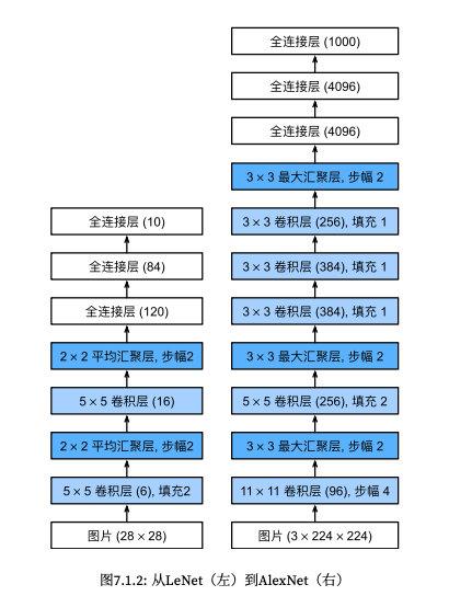
image_1661567510569_0

```
          AlexNet(
            (features): Sequential(
              (0): Conv2d(3, 64, kernel_size=(11, 11), stride=(4, 4), padding=(2, 2))
              (1): ReLU(inplace=True)
              (2): MaxPool2d(kernel_size=3, stride=2, padding=0, dilation=1, ceil_mode=False)
              (3): Conv2d(64, 192, kernel_size=(5, 5), stride=(1, 1), padding=(2, 2))
              (4): ReLU(inplace=True)
              (5): MaxPool2d(kernel_size=3, stride=2, padding=0, dilation=1, ceil_mode=False)
              (6): Conv2d(192, 384, kernel_size=(3, 3), stride=(1, 1), padding=(1, 1))
              (7): ReLU(inplace=True)
              (8): Conv2d(384, 256, kernel_size=(3, 3), stride=(1, 1), padding=(1, 1))
              (9): ReLU(inplace=True)
              (10): Conv2d(256, 256, kernel_size=(3, 3), stride=(1, 1), padding=(1, 1))
              (11): ReLU(inplace=True)
              (12): MaxPool2d(kernel_size=3, stride=2, padding=0, dilation=1, ceil_mode=False)
            )
            (avgpool): AdaptiveAvgPool2d(output_size=(6, 6))
            (classifier): Sequential(
              (0): Dropout(p=0.5, inplace=False)
              (1): Linear(in_features=9216, out_features=4096, bias=True)
              (2): ReLU(inplace=True)
              (3): Dropout(p=0.5, inplace=False)
              (4): Linear(in_features=4096, out_features=4096, bias=True)
              (5): ReLU(inplace=True)
              (6): Linear(in_features=4096, out_features=1000, bias=True)
            )
          )
  ```
class AlexNet(nn.Module):
    def __init__(self, num_classes=1000, init_weights=False):
        super(AlexNet, self).__init__()
        self.features = nn.Sequential(
            nn.Conv2d(3, 64, kernel_size=11, stride=4, padding=2),
            nn.ReLU(inplace=True),
            nn.MaxPool2d(kernel_size=3, stride=2),
            nn.Conv2d(64, 192, kernel_size=5, padding=2),
            nn.ReLU(inplace=True),
            nn.MaxPool2d(kernel_size=3, stride=2),
            nn.Conv2d(192, 384, kernel_size=3, padding=1),
            nn.ReLU(inplace=True),
            nn.Conv2d(384, 256, kernel_size=3, padding=1),
            nn.ReLU(inplace=True),
            nn.Conv2d(256, 256, kernel_size=3, padding=1),
            nn.ReLU(inplace=True),
            nn.MaxPool2d(kernel_size=3, stride=2),
        )
        self.avgpool = nn.AdaptiveAvgPool2d((6, 6))
        self.classifier = nn.Sequential(
            nn.Dropout(),
            nn.Linear(256 * 6 * 6, 4096),
            nn.ReLU(inplace=True),
            nn.Dropout(),
            nn.Linear(4096, 4096),
            nn.ReLU(inplace=True),
            nn.Linear(4096, num_classes),
        )
        if init_weights:
            self._initialize_weights()

    def forward(self, x):
        x = self.features(x)
        x = torch.flatten(x, start_dim=1)
        x = self.classifier(x)
        return x

    def _initialize_weights(self):
        for m in self.modules():
            if isinstance(m, nn.Conv2d):
                nn.init.kaiming_normal_(m.weight, mode='fan_out', nonlinearity='relu')
                if m.bias is not None:
                    nn.init.constant_(m.bias, 0)
            elif isinstance(m, nn.Linear):
                nn.init.normal_(m.weight, 0, 0.01)
                nn.init.constant_(m.bias, 0)

```

特点

因为在两块GPU上运行，因此网络结构被一分为二
五层 convolutional layers加上三层 fullyconnected layers
2，4，5层仅与自己之前的核有关系，也就是仅与自己这个GPU前一层训练的输出有关，第三层与前一层的两个GPU有关，在通道上做了一层融合
Local Response Normalization运用在第一层和第二层
每一层都使用了 ReLu

0x04 Reducing overfitting

4.1 Data Augmentation

这里的输入是256*256，但是网络的输入是224*224，因为为了扩充数据集的大小，在之后的训练过程中可以随机选择，这样可以得到2^11=2048倍的扩充
另外一种方法是使用PCA对RGB进行修正，是的数据的数量得到增多，最终的效果也是成功的

4.2 dropout

0.5的概率将一些神经元的输出设置为0，可以有效的降低过拟合

0x05 Details of learning

SGD，随机梯度下降，增加动量的选项 初始化参数，使用均值为0、方差为0.01的高斯随机变量初始化权重参数 LearningRate设置为0.01

0x06 Results

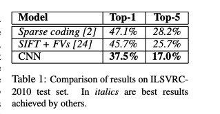
image_1661568191988_0

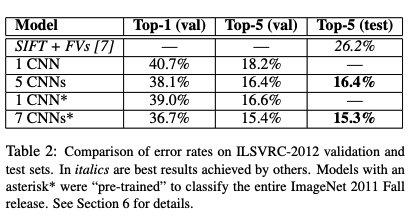
image_1661568198286_0

0x07 参考别人的复现

to be continued ~~