defgenerate_index_map(labels): index2label = {} label2index = {} i = 0 for label in labels: index2label[i] = label label2index[label] = i i += 1 return index2label,label2index
defgen_Pi(pi_dict,Qlabel): v = np.zeros(len(Qlabel),dtype=float) for key in pi_dict: v[Qlabel[key]] = pi_dict[key] return v
defgen_matrix(trans_dict,Qlabel,Vlabel): res = np.zeros((len(Qlabel),len(Vlabel)),dtype=float) for si in trans_dict: for sj in trans_dict[si]: res[Qlabel[si]][Vlabel[sj]] = trans_dict[si][sj] return res
A = gen_matrix(A,Qindex,Qindex) B = gen_matrix(B,Qindex,Vindex) pi = gen_Pi(Pi,Qindex) print('state transition matrix') print(A) print('state-observation matrix') print(B) print('state prob distribution') print(pi)
之后我们来模拟生成
1
2
3
4
5
6
7
8
9
10
11
12
13
14
15
16
def simulate(T,A,B,pi):
    def draw_from(state_prob_distribution):
        return np.where(np.random.multinomial(1,state_prob_distribution)==1)[0][0]
    observations = np.zeros(T,dtype=int)
    states = np.zeros(T,dtype=int)
    states[0] = draw_from(pi)
    observations[0] = draw_from(B[states[0],:])
    for t in range(1, T):
        states[t] = draw_from(A[states[t-1],:])
        observations[t] = draw_from(B[states[t],:])
    return observations, states

# simulate the data
O,I = simulate(10,A,B,pi)
print([Qlabel[i] for i in I])
print([Vlabel[j] for j in O])
# In the study of HMM, there are three main problems # Track Probability: give the O={o1,o2,...,oT},P(O) # Learning problem: give the O, estimate the parameters # Forecasting problem: (decoding problem also),given the observation track, # show the most likely state track
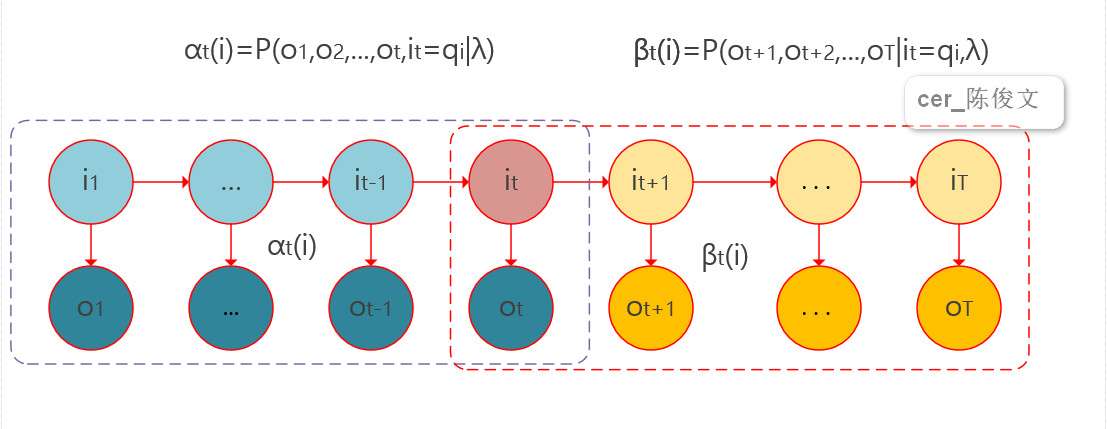
defforward(obs_seq,A,B,pi): '''cal the probability from the observation sequence with forward''' state_len = A.shape[0] track_len = len(obs_seq) F = np.zeros((state_len,track_len))
# init the state with the pi F[:,0] = pi*B[:,obs_seq[0]] for t inrange(1,track_len): for n inrange(state_len): F[n,t] = np.dot(F[:,t-1],(A[:,n]))*B[n,obs_seq[t]] return F
defbackward(obs_seq,A,B,pi): '''cal the probability from the observation sequence with backward''' N = A.shape[0] T = len(obs_seq) # X保存后向概率矩阵 X = np.zeros((N,T)) X[:,-1:] = 1
for t inreversed(range(T-1)): for n inrange(N): X[n,t] = np.sum(X[:,t+1] * A[n,:] * B[:, obs_seq[t+1]])
return X
print('track probability forward') print(forward(O,A,B,pi)) print('track probability backward') print(backward(O,A,B,pi))
# Based on the EM algrithm, the HMM learning process can be solved by Baum-Weich algorithm def baum_weich(obs_seq,A,B,pi,criterion=0.05): ''' Unsupervised learning algorithm ''' n_states = A.shape[0] n_samples = len(obs_seq)
done = False
whilenot done: # Cal the track probability # alpha(i) = p(obs_seq | q0=s_i,hmm) alpha = forward(obs_seq,A,B,pi) # beta(i)=p(obs_seq | q0=s_i,hmm) beta = backward(obs_seq,A,B,pi)
# xi: in the timestamp t, the t state is i and the t+1 state is j xi = np.zeros((n_states,n_states,n_samples-1)) for t inrange(n_samples-1): denom = np.dot(np.dot(alpha[:,t].T, A) * B[:,obs_seq[t+1]].T, beta[:,t+1]) for i inrange(n_states): numer = alpha[i,t] * A[i,:] * B[:,obs_seq[t+1]].T * beta[:,t+1].T xi[i,:,t] = numer / denom
# gamma, in the timestamp t ,the t state is i gamma = np.sum(xi,axis=1) # prod for what prod = (alpha[:,n_samples-1]*beta[:,n_samples-1]).reshape((-1,1)) gamma = np.hstack((gamma,prod/np.sum(prod)))
defviterbi(obs_seq, A, B, pi): """ Returns ------- V : numpy.ndarray V [s][t] = Maximum probability of an observation sequence ending at time 't' with final state 's' prev : numpy.ndarray Contains a pointer to the previous state at t-1 that maximizes V[state][t]
V对应δ,prev对应ψ """ N = A.shape[0] T = len(obs_seq) prev = np.zeros((T - 1, N), dtype=int)
# DP matrix containing max likelihood of state at a given time V = np.zeros((N, T)) V[:,0] = pi * B[:,obs_seq[0]]
for t inrange(1, T): for n inrange(N): seq_probs = V[:,t-1] * A[:,n] * B[n, obs_seq[t]] prev[t-1,n] = np.argmax(seq_probs) V[n,t] = np.max(seq_probs)
return V, prev
defbuild_viterbi_path(prev, last_state): """Returns a state path ending in last_state in reverse order. 最优路径回溯 """ T = len(prev) yield(last_state) for i inrange(T-1, -1, -1): yield(prev[i, last_state]) last_state = prev[i, last_state]
defobservation_prob(obs_seq): """ P( entire observation sequence | A, B, pi ) """ return np.sum(forward(obs_seq)[:,-1])
defstate_path(obs_seq, A, B, pi): """ Returns ------- V[last_state, -1] : float Probability of the optimal state path path : list(int) Optimal state path for the observation sequence """ V, prev = viterbi(obs_seq, A, B, pi) # Build state path with greatest probability last_state = np.argmax(V[:,-1]) path = list(build_viterbi_path(prev, last_state))
import torch import torch.autograd as autograd import torch.nn as nn import torch.optim as optim torch.manual_seed(2023)
# Define the helper functions to make the code more readable defargmax(vector): ''' return the argmax index ''' _, idx = torch.max(vector,1) return idx.item()
defprepare_sequence(seq,to_ix): idxs = [to_ix[w] for w in seq] return torch.tensor(idxs,dtype=torch.long)
deflog_sum_exp(vector): ''' return the log sum exp in a numerically stable way fot the forward algorithm ''' max_score = vector[0,argmax(vector)] max_score_broadcast = max_score.view(1,-1).expand(1,vector.size()[1]) return max_score+torch.log(torch.sum(torch.exp(vector-max_score_broadcast)))
# Maps the output of the LSTM into tag space. self.hidden2tag = nn.Linear(hidden_dim, self.tagset_size)
# Matrix of transition parameters. Entry i,j is the score of # transitioning *to* i *from* j. self.transitions = nn.Parameter( torch.randn(self.tagset_size, self.tagset_size))
# These two statements enforce the constraint that we never transfer # to the start tag and we never transfer from the stop tag self.transitions.data[tag_to_ix[START_TAG], :] = -10000 self.transitions.data[:, tag_to_ix[STOP_TAG]] = -10000
def_forward_alg(self, feats): # Do the forward algorithm to compute the partition function init_alphas = torch.full((1, self.tagset_size), -10000.) # START_TAG has all of the score. init_alphas[0][self.tag_to_ix[START_TAG]] = 0.
# Wrap in a variable so that we will get automatic backprop forward_var = init_alphas
# Iterate through the sentence for feat in feats: alphas_t = [] # The forward tensors at this timestep for next_tag inrange(self.tagset_size): # broadcast the emission score: it is the same regardless of # the previous tag emit_score = feat[next_tag].view( 1, -1).expand(1, self.tagset_size) # the ith entry of trans_score is the score of transitioning to # next_tag from i trans_score = self.transitions[next_tag].view(1, -1) # The ith entry of next_tag_var is the value for the # edge (i -> next_tag) before we do log-sum-exp next_tag_var = forward_var + trans_score + emit_score # The forward variable for this tag is log-sum-exp of all the # scores. alphas_t.append(log_sum_exp(next_tag_var).view(1)) forward_var = torch.cat(alphas_t).view(1, -1) terminal_var = forward_var + self.transitions[self.tag_to_ix[STOP_TAG]] alpha = log_sum_exp(terminal_var) return alpha
# Initialize the viterbi variables in log space init_vvars = torch.full((1, self.tagset_size), -10000.) init_vvars[0][self.tag_to_ix[START_TAG]] = 0
# forward_var at step i holds the viterbi variables for step i-1 forward_var = init_vvars for feat in feats: bptrs_t = [] # holds the backpointers for this step viterbivars_t = [] # holds the viterbi variables for this step
for next_tag inrange(self.tagset_size): # next_tag_var[i] holds the viterbi variable for tag i at the # previous step, plus the score of transitioning # from tag i to next_tag. # We don't include the emission scores here because the max # does not depend on them (we add them in below) next_tag_var = forward_var + self.transitions[next_tag] best_tag_id = argmax(next_tag_var) bptrs_t.append(best_tag_id) viterbivars_t.append(next_tag_var[0][best_tag_id].view(1)) # Now add in the emission scores, and assign forward_var to the set # of viterbi variables we just computed forward_var = (torch.cat(viterbivars_t) + feat).view(1, -1) backpointers.append(bptrs_t)
# Follow the back pointers to decode the best path. best_path = [best_tag_id] for bptrs_t inreversed(backpointers): best_tag_id = bptrs_t[best_tag_id] best_path.append(best_tag_id) # Pop off the start tag (we dont want to return that to the caller) start = best_path.pop() assert start == self.tag_to_ix[START_TAG] # Sanity check best_path.reverse() return path_score, best_path
defneg_log_likelihood(self, sentence, tags): # Input the sentence with the dirsed tags feats = self._get_lstm_features(sentence) # Cancaluate the feature from the lsmt layers print('FEAT',feats) forward_score = self._forward_alg(feats) # Calculante the forward scoress, based on the feats print('FORWARD_SCORE',forward_score) gold_score = self._score_sentence(feats, tags) # calculate the score from the sentence return forward_score - gold_score
defforward(self, sentence): # dont confuse this with _forward_alg above. # Get the emission scores from the BiLSTM lstm_feats = self._get_lstm_features(sentence)
# Find the best path, given the features. score, tag_seq = self._viterbi_decode(lstm_feats) return score, tag_seq
# Training process START_TAG = '<START>' STOP_TAG = '<STOP>' EMBEDDING_DIM = 5 HIDDEN_DEM = 4
# Makding up the training data training_data = [ ( "the wall street journal reported today that apple corporation made money".split(), "B I I I O O O B I O O".split()), ( "georgia tech is a university in georgia".split(), "B I O O O O B".split() ) ] word_to_ix = {} for sentence,tags in training_data: for word in sentence: if word notin word_to_ix: word_to_ix[word] = len(word_to_ix)
with torch.no_grad(): precheck_sent = prepare_sequence(training_data[0][0],word_to_ix) precheck_tags = torch.tensor([tag_to_ix[t] for t in training_data[0][1]],dtype=torch.long)
# Make sure prepare_sequence from earlier in the LSTM section is loaded for epoch inrange(300): # again, normally you would NOT do 300 epochs, it is toy data for sentence, tags in training_data: # Step 1. Remember that Pytorch accumulates gradients. # We need to clear them out before each instance model.zero_grad()
# Step 2. Get our inputs ready for the network, that is, # turn them into Tensors of word indices. sentence_in = prepare_sequence(sentence, word_to_ix) targets = torch.tensor([tag_to_ix[t] for t in tags], dtype=torch.long)
# Step 3. Run our forward pass. loss = model.neg_log_likelihood(sentence_in, targets)
# Step 4. Compute the loss, gradients, and update the parameters by # calling optimizer.step() loss.backward() optimizer.step()
# Check predictions after training with torch.no_grad(): precheck_sent = prepare_sequence(training_data[0][0], word_to_ix) print(model(precheck_sent))